


It is a period of uneasy peace. The phantom pressure has been exposed and the bathtub drained. Yet one relic of the old order remains: an equation that continues to balance even after its mechanism has failed…
The equation that refused to die
After decades of debate, the classical explanation of venous return was in serious trouble.
Mean systemic filling pressure, Pms, had no demonstrated anatomical location during flow. Right atrial pressure was not an independent back pressure controlling how much blood returned to the heart. The venous system could store elastic energy and release some of it during transitions, but it could not supply the continuing energy required for steady flow.
The bathtub had provided a memorable picture containing some useful insights. Unfortunately, its gravitational energy source belonged to the bathtub rather than the circulation.
Yet the equation remained:
where Q is systemic blood flow, PRA is right atrial pressure and RVR is the so-called resistance to venous return.
Guyton’s equation fitted his experimental data. It still appeared in textbooks. Clinicians used it to think about fluids, vasopressors and cardiac function. Even critics who rejected its usual interpretation accepted that the mathematics was correct.
This presented a difficult question. How could an equation containing a pressure defined when flow had stopped describe a circulation in which blood was still moving?
In 2011, Daniel Beard and Eric Feigl returned to Guyton’s original model and worked through its mathematics. They were not proposing an entirely new explanation. Levy had already corrected the direction of dependency. Rothe had described the passive redistribution of blood between vascular compartments, and Brengelmann had used that redistribution to challenge the back-pressure interpretation of right atrial pressure. Beard and Feigl brought these earlier arguments together and showed how they were already encoded within Guyton’s own model. The equation was valid, but it did not mean what generations of physiologists had assumed.
To understand why, we need to rebuild the model from its component parts.
Starting the pump
Beard and Feigl depicted the systemic circulation using two elastic compartments.
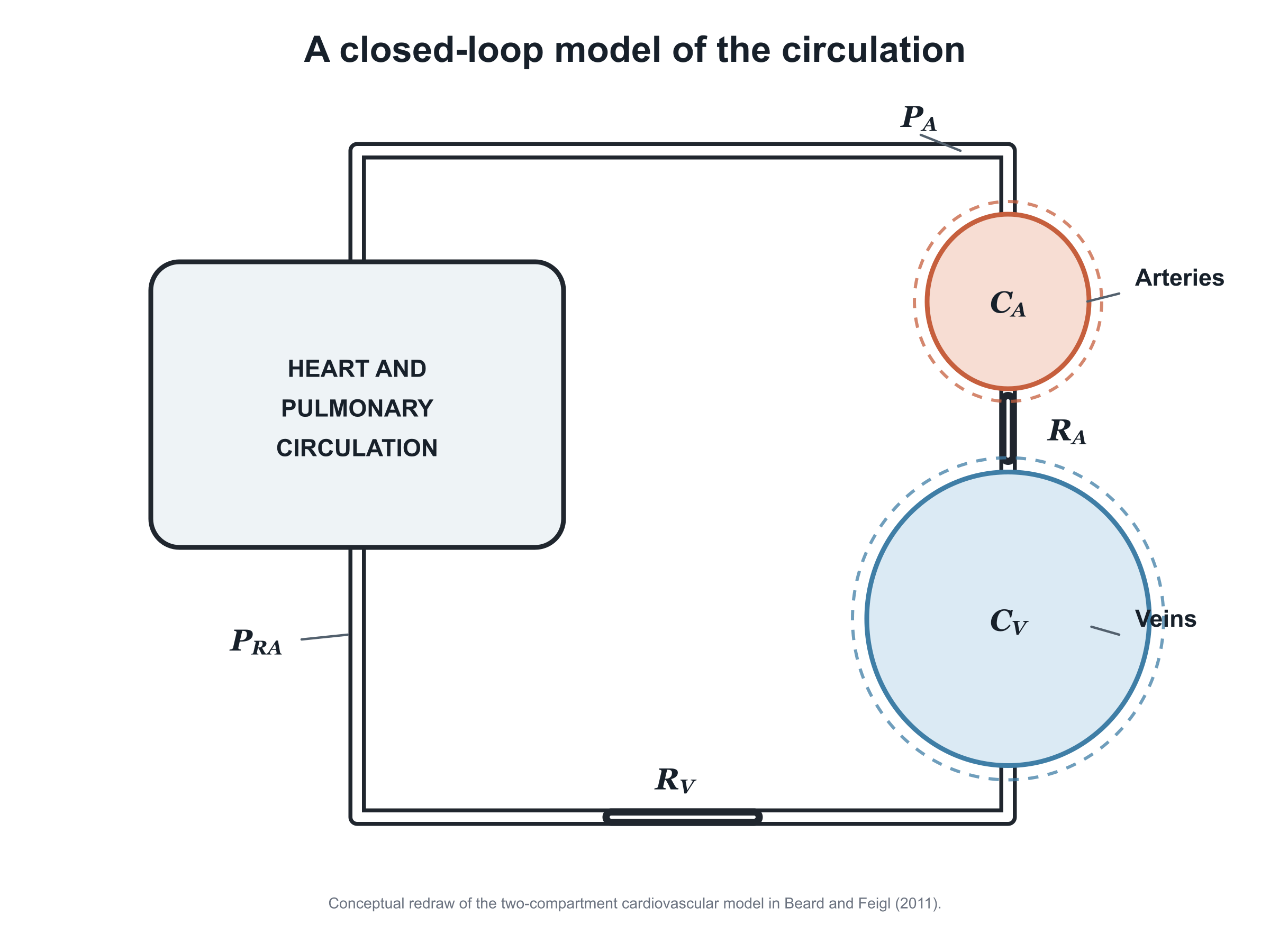
One represented the arteries. The other represented the veins. Each could expand as it contained more blood. Physical resistances separated the compartments, and a pump transferred blood from the venous side back into the arterial side.
Begin with the pump stopped. There is no flow, so the pressure differences across the resistances disappear. Blood redistributes between the arterial and venous compartments until they reach a common equilibrium pressure. That pressure is mean systemic filling pressure.
Now start the pump. Blood is transferred into the arterial compartment faster than it initially leaves. Its contained volume rises, its walls distend and arterial pressure rises. Because total systemic blood volume is fixed, the additional arterial volume comes from the venous side. The veins contain less blood and their pressure falls. Right atrial pressure falls as part of this redistribution.
After a short transition, flow through every part of the system becomes equal again. Blood continues to circulate, but the average volume contained within each compartment is now stable. This is a flowing steady state. Steady does not mean stationary. It means that each compartment receives and loses blood at the same average rate, so its contained volume no longer changes.
The pump has established a new pressure and volume distribution. Arterial pressure lies above the original equilibrium pressure, while venous and right atrial pressures lie below it. The actual pressure difference across the systemic circulation is:
where (Pa) is mean arterial pressure and (Rt) is total systemic vascular resistance.
Both pressures exist while blood is flowing. They lie at identifiable points on the same vascular pathway. The heart supplies the energy, and blood loses mechanical energy as it passes through the intervening resistance.
No compartment maintained at Pms is required.
The zero-flow intercept
Guyton did not measure one flowing state. He imposed several different pump flows and allowed the circulation to settle after each adjustment.
Each flow produced a different distribution of the same total blood volume. At higher flows, more blood resided on the arterial side and less remained in the veins. Arterial pressure rose while right atrial pressure fell.
These were separate steady states of the same vascular system. Total blood volume, vascular resistance and vascular compliance were held constant. Only the imposed flow and the resulting pressure-volume distribution changed.
If flow is plotted on the vertical axis and right atrial pressure on the horizontal axis, the points form a descending line. When flow reaches zero, right atrial pressure reaches Pms. Mean systemic filling pressure is therefore the zero-flow intercept of the relationship.
An illustrative set of values makes this easier to see.
Imagine four steady states:
At an imposed flow of 0 L/min, RAP is 10 mmHg.
At 1 L/min, RAP is 8 mmHg.
At 2 L/min, RAP is 6 mmHg.
At 3 L/min, RAP is 4 mmHg.
These are four separate steady states. At each flowing state, blood is moving at the same rate through every part of the circuit and the average volume of each compartment is stable.
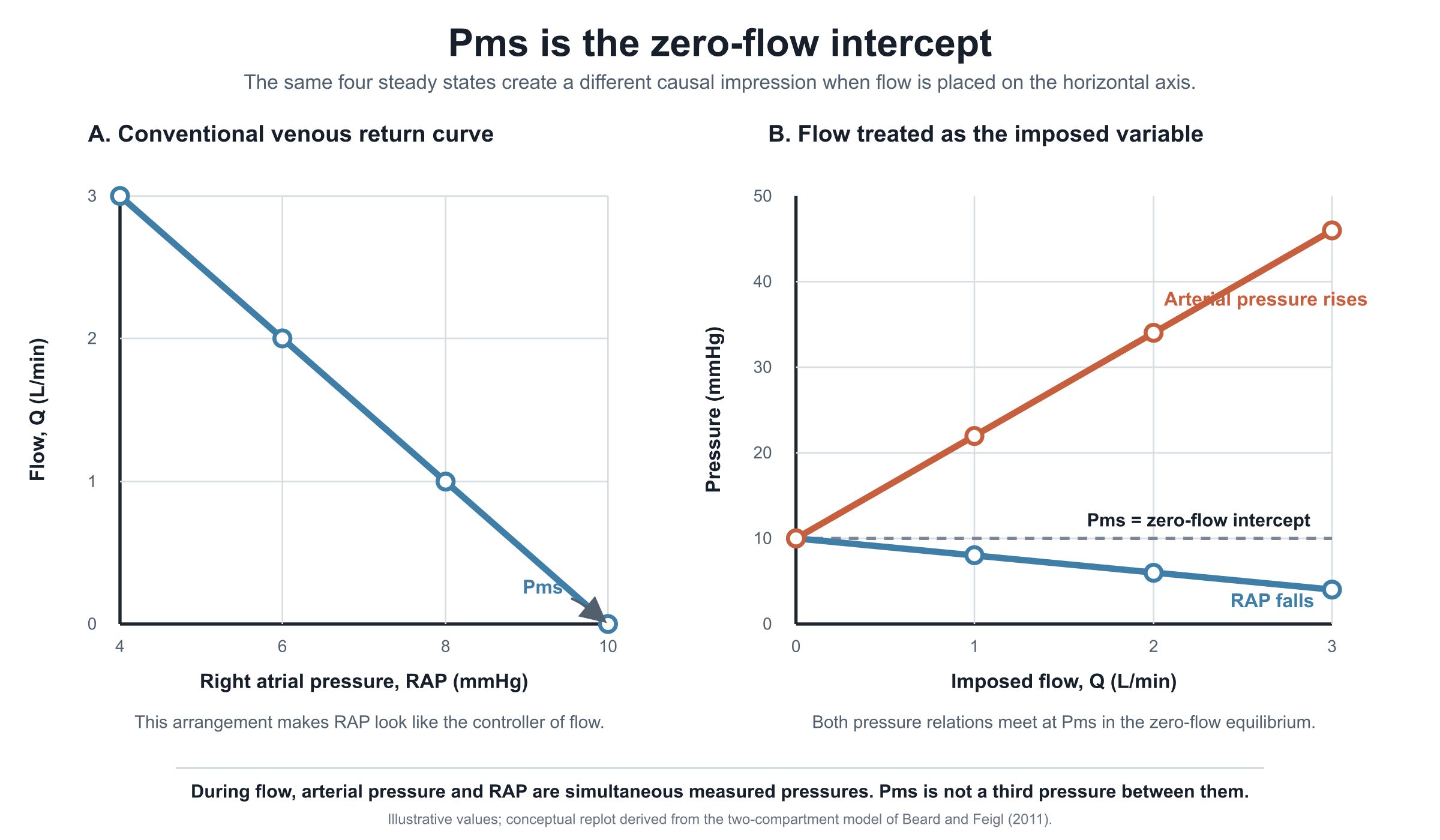
When flow is zero, right atrial pressure is 10 mmHg. This is the zero-flow intercept, Pms. For every 1 L/min increase in imposed flow, right atrial pressure falls by 2 mmHg as blood is redistributed from the venous compartment to the arterial compartment.
The equation can therefore be written:
At a flow of 2 L/min, right atrial pressure is 6 mmHg. The value 10 mmHg does not represent an upstream pressure acting on the right atrium during that flowing state. It tells us only that right atrial pressure now lies 4 mmHg below the value it would have at zero flow.
Replacing 10 with Pms, and replacing the slope of 2 with RVR, gives:
Rearranging the same line produces the familiar Guyton equation:
The rearrangement changes how the equation looks. It does not turn the zero-flow intercept into a physical upstream pressure.
Another way to think about it:
For a moment, forget the name Pms and call this intercept P0. The line can then be written:
where K is the slope relating a change in flow to the resulting change in right atrial pressure.
Read this from left to right:
Current right atrial pressure equals its zero-flow value minus the change associated with flow-driven redistribution of blood volume.
There is no suggestion that blood flows from P0. It is simply the value that right atrial pressure would reach if flow returned to zero.
In Guyton’s model, P0 is mean systemic filling pressure. The equation therefore becomes:
A uniform pressure equal to Pms exists physically only after flow has stopped and the systemic pressures have equilibrated. Its value can nevertheless be defined while flow continues. The blood volume and vascular properties that would determine the equilibrium pressure still exist.
A visual analogy:
Imagine two tanks containing a fixed amount of water. A pump maintains one water level above the other. If the pump stops and the tanks are connected, the water will settle at a common level. That future equilibrium level is not currently present in either tank, but it can still be calculated from the total volume of water and the dimensions of the tanks.
Mean systemic filling pressure has the same status during flow. It is the pressure the vascular system would reach if the pump stopped without any change in blood volume or vascular tone. It appears in the equation as a reference value. It is not an upstream pressure within the flowing circulation.
A resistance containing compliance
The denominator presents another puzzle.
Guyton’s original term for it was not resistance to venous return. In 1955, he wrote that it depended on the resistance and capacitance of different parts of the peripheral circulation. He called it the impedance to venous return.
That name contained an important warning. Guyton was not describing a single venous resistor lying between Pms and the right atrium. He was combining the effects of the whole vascular network into one quantity.
He was using impedance broadly. In its modern technical sense, impedance describes the relationship between pulsatile pressure and flow and may include resistance, compliance, inertance, frequency and timing. Guyton’s equation related steady states, so this was not impedance in its complete modern sense. Even so, the term was more informative than the later resistance to venous return, because it signalled that resistance alone was not enough.
Beard and Feigl showed that the quantity later called resistance to venous return was:
Where RV and RA are venous and arterial resistance, while CV and CA are venous and arterial compliance.
At first sight, this looks like a resistance containing compliance. But physical resistance does not contain compliance. Resistance dissipates mechanical energy as blood flows through a vessel. Compliance describes how much volume a vascular compartment stores as its pressure changes.
The compliance ratio in the equation has no units, so RVR retains the units of resistance. That does not make it a physical resistor. It is a calculated slope describing how much right atrial pressure changes when imposed flow changes between steady states.
That response depends on the whole vascular system.
When Guyton increased pump flow, blood was transferred into the arterial compartment. Passing the greater flow through the arterial resistance required a larger pressure difference. Because the arterial compartment was compliant, its higher pressure was accompanied by a greater contained volume. Total systemic blood volume was fixed, so this additional arterial volume came from the venous compartment. Venous volume and right atrial pressure therefore fell.
The pump transferred the blood. Resistance helped determine how much the arterial pressure and volume had to rise before the imposed flow could pass through the compartment.
Compliance was essential to this response. If the arterial compartment had been completely rigid, its pressure could have risen without storing additional blood. No extra volume would then have been removed from the veins for arterial storage. If there had been no arterial resistance, no additional pressure difference or arterial expansion would have been required for blood to leave the compartment.
Venous compliance also affected the result. A given loss of venous volume produces a smaller fall in right atrial pressure when the venous compartment is highly compliant than when it is stiff. The slope therefore depends on how compliance is distributed between the arterial and venous sides, as well as on their physical resistances.
This is why RVR can differ greatly from the actual venous resistance. Under some plausible assumptions, arterial resistance makes the larger contribution.
The term resistance to venous return conceals all of this. It encourages the reader to imagine a resistor situated between Pms and the right atrium. Guyton’s earlier impedance to venous return was better, although still incomplete. The most exact description would be the slope coefficient of the venous return curve: a composite measure of how resistance, compliance and conservation of blood volume relate imposed flow to right atrial pressure.
Once the denominator is understood this way, the equation looks rather less like Ohm’s law across a physical venous pathway.
Turning the equation around
The familiar form of Guyton’s equation reads:
Its arrangement suggests a causal story. A higher upstream pressure, a lower downstream pressure and a resistance between them. The pressure difference appears to produce the flow.
But the same equation can be rearranged:
It now suggests that the pressure gradient is caused by flow through the vascular system.
In Guyton’s experiments, this was the direction of the intervention. The pump imposed flow. Blood moved from the venous compartment into the arterial compartment and right atrial pressure fell below its zero-flow value.
The equation itself contains no arrow of causation. Its arrangement merely encourages us to infer one.
Beard and Feigl made the problem even clearer by writing an equivalent equation from the arterial side of the same model:
where Ct is total systemic compliance.
This equation is just as valid as the venous return equation. Yet if its arrangement were interpreted causally, Pms would become a back pressure opposing arterial delivery. Lowering Pms would appear to increase cardiac output
No one interprets it this way.
Both equations emerge from the same physical resistances, compliant compartments and conservation of blood volume. One is written relative to right atrial pressure and the other relative to arterial pressure. Neither identifies a hidden motor.
If the position of a term within an equation established causality, Pms could be made to promote venous return in one arrangement and oppose arterial delivery in another.
The Guyton equation resembles Ohm’s law because it can be written in the form ΔP = QR. Its terms do not carry the same physical meaning.
The quantity Pms − Pra is not the pressure difference between two locations in the flowing circulation. It is the difference between the current right atrial pressure and its zero-flow reference value.
The quantity Rvr is not the physical resistance connecting those pressures. It is the slope relating flow to the redistribution of pressure and volume across the whole vascular system.
The equation is valid as vascular bookkeeping. It fails when treated as a mechanism of propulsion.
Should the curve still be taught?
Once the equation had been separated from its usual physical interpretation, a further question remained. Was the venous return curve still a useful way to teach the circulation?
The Journal of Physiology debated this directly in 2013. Philip Andrew accepted the central criticisms of Guyton’s interpretation. Flow had been imposed in the original experiments, right atrial pressure was not the independent variable, and Pms − Pra was not the physical pressure gradient for systemic blood flow. He nevertheless argued that Guyton’s graphical analysis remained valuable. The vascular curve could be reinterpreted as a venous pressure curve, showing how right atrial pressure changed when flow was imposed. Its intersection with the cardiac function curve would still identify the flow and right atrial pressure compatible with both the heart and the vascular system.
Beard and Feigl thought the confusion was too deeply embedded to be repaired by renaming the curve. Right atrial pressure remained on the conventional horizontal axis, encouraging it to be read as the independent controller of venous return. The zero-flow intercept still looked like an upstream pressure source, and the slope still looked like a physical resistance leading to the right atrium. They concluded that the curve generated more misunderstanding than insight and should no longer be taught.
I think they were right.
Guyton’s operating-point insight remains important. The heart and vascular system cannot independently select their own flow and pressure. The circulation must settle on a state compatible with cardiac acceptance and ejection, blood volume, vascular accommodation and resistance.
None of this requires a venous return curve.
If cardiovascular physiology were being constructed from first principles today, we would begin with the heart, the blood it moves and the vessels through which it moves. Resistance, compliance, blood volume and conservation would come before mean systemic filling pressure or right atrial pressure. Those pressures would be introduced later as measurements of the circulatory state, rather than as the two ends of a pressure gradient.
If Guyton’s venous return curve wasn’t so ubiquitous, no one attempting to teach the circulation from first principles would use it today.
Its remaining educational value is historical. It shows how a mathematically correct relationship can acquire an incorrect physical explanation, particularly when the arrangement of a graph encourages the reader to mistake a dependent variable for a cause.
Does the equation survive?
Guyton’s equation is not meaningless.
Within its assumptions, it describes a family of steady states in a simplified vascular system. It tells us how imposed flow redistributes a fixed blood volume and how right atrial pressure changes as part of that redistribution. It identifies the zero-flow equilibrium pressure associated with the vascular state. It shows which combinations of flow and right atrial pressure are compatible with the model.
It does not show where the energy for flow originates. It does not identify a pathway running from Pms to the right atrium. It does not make right atrial pressure an independent controller of venous return. Its denominator does not correspond to a resistance located in the veins. Nor can the equation decide what cardiac output the intact circulation will establish.
Beard and Feigl concluded: ‘Guyton’s idea, that venous return (equal to cardiac output) is determined by the pressure difference between mean systemic pressure and right atrial pressure (Pms – Pra) is physically and physiologically wrong’. I agree and would argue that its remaining educational value is historical: it shows how valid mathematics, arranged in a familiar form, can acquire a physical meaning that the underlying model does not support.
There remains one final problem. The Guytonian framework remains clinically persuasive because many of its predictions appear to work. Magder gave that framework its most intuitive modern form through the bathtub analogy. Guyton’s intersecting curves had already shown that the heart and vasculature constrain each other. Magder made the division more explicit: once the heart can accept and replace the blood presented to it, further cardiac power achieves little unless vascular delivery also changes.
This seems to fit clinical experience. Fluids and vasopressors can increase cardiac output. Poor cardiac function produces congestion. Once cardiac function is no longer limiting, additional cardiac power often achieves little.
If Pms does not push blood towards the heart, why does increasing the vascular elastic state so often increase cardiac output? If RAP does not oppose venous return, why does a high RAP so often accompany circulatory failure? Why can the same intervention increase flow in one patient while producing only higher pressures in another?
The critics have shown why the old physical explanation cannot be right. They have been less successful at replacing the clinically useful model built upon it.
Yet the pieces of that replacement have been present throughout this series: Guyton’s coupled circulation, Levy’s dependent variables, Rothe’s elastic state, Brengelmann’s energy analysis, Magder’s clinical constraints and Beard’s surviving equation.
In the final episode, I will bring those pieces together. The aim is no longer to decide whether the heart or the vasculature controls cardiac output. It is to explain how cardiac energy, vascular delivery and cardiac acceptance resolve into one flowing state, why familiar treatments work, and why they sometimes fail.
Dismantling the old model was only the beginning.
The war has cleared the ground. It is time to rebuild the circulation.
Next: Episode VIII — The Dependent Variable
References
Andrew P. CrossTalk proposal: Guyton’s venous return curves should be taught. J Physiol. 2013;591:5791–5793.
Beard DA, Feigl EO. Understanding Guyton’s venous return curves. Am J Physiol Heart Circ Physiol. 2011;301–H633.
Beard DA, Feigl EO. CrossTalk opposing view: Guyton’s venous return curves should not be taught. J Physiol. 2013;591:5795–5797.
Guyton AC. Determination of cardiac output by equating venous return curves with cardiac response curves. Physiol Rev. 1955;35:123–129.
Levy MN. The cardiac and vascular factors that determine systemic blood flow. Circ Res. 1979;44:739–747.